Vector Databases and Embeddings Explained

Traditional relational databases and search engines were engineered to answer deterministic questions: Does this user ID match? Does this column fall between two timestamps? Does this document contain the exact term "database"? These queries rely on scalar comparisons, B-trees, hash maps, and inverted indexes built on discrete lexical tokens.

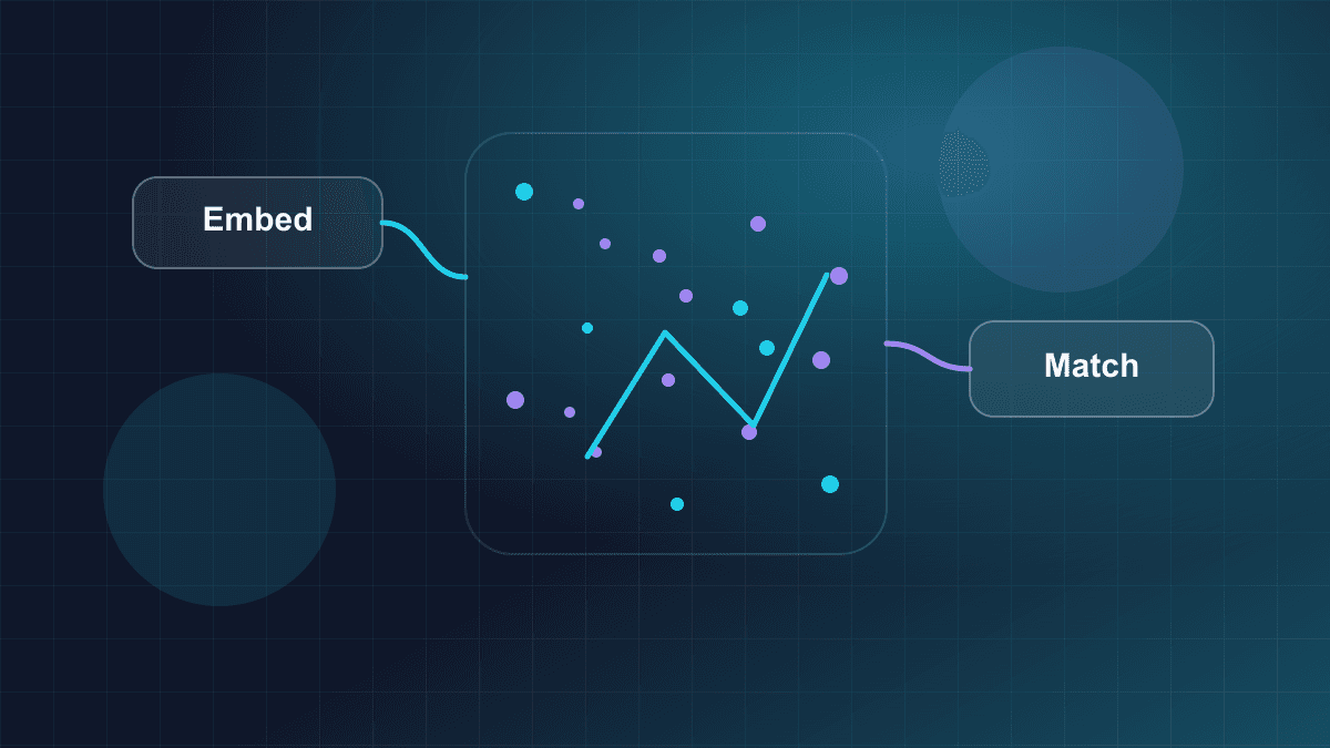
Modern artificial intelligence workflows—such as semantic search, retrieval-augmented generation (RAG), recommendation engines, and multimodal classification—operate on fundamentally different data. Machine learning models represent text, images, audio, and graph entities not as discrete strings, but as dense numerical arrays called vector embeddings.

Searching through millions of high-dimensional vectors to identify semantically related items cannot be achieved using standard relational indexes. Doing so requires specialized spatial indexing algorithms, geometric distance calculations, and purpose-built vector databases.

This guide explores the architecture of vector databases and embeddings from an engineering perspective: the underlying mathematical principles, Approximate Nearest Neighbor (ANN) indexing structures, the operational tradeoffs between dedicated vector engines and vector-extended relational databases, metadata filtering dilemmas, and concrete production implementation patterns.

---

1. Mathematical Foundations of Vector Embeddings

What Is a Vector Embedding?

Mathematically, a vector embedding is a mapping function $f: \mathcal{X} \to \mathbb{R}^D$ that projects an arbitrary input object $x \in \mathcal{X}$ (such as a passage of text, a code snippet, or an image) into a $D$-dimensional continuous vector space.

Input Text / Chunk
"PostgreSQL transaction isolation"
                │
                ▼ Embedding Model (e.g., text-embedding-3-small)
   [0.0142, -0.0521, 0.0891, ..., -0.0034]  ∈  ℝ^1536

The dimension $D$ typically ranges from 384 to 3072 in modern transformer architectures. In this latent space, semantic proximity translates to geometric proximity: vectors representing concepts with similar semantic meanings reside close to one another, while unrelated concepts are separated by larger geometric distances.

Vector Distance and Similarity Metrics

To evaluate whether two items are semantically related, a database calculates the geometric distance or similarity between their embedding vectors $u, v \in \mathbb{R}^D$. Three primary metrics dominate production vector search:

1. Euclidean Distance ($L_2$ Norm)

Euclidean distance measures the straight-line geometric distance between two coordinate points in $D$-dimensional space:

$\|u - v\|_2 = \sqrt{\sum_{i=1}^D (u_i - v_i)^2}$

Euclidean distance is sensitive to vector magnitude. If two text passages have identical semantic topic distributions but differing lengths, an unnormalized model might scale their magnitudes differently, resulting in an artificially large Euclidean distance.

2. Dot Product (Inner Product)

The dot product measures both the angle between vectors and their relative magnitudes:

$\langle u, v \rangle = u \cdot v = \sum_{i=1}^D u_i v_i$

Dot product is widely used in recommendation systems where vector magnitude encodes item popularity or user preference intensity.

3. Cosine Similarity and Cosine Distance

Cosine similarity isolates the directional angle between two vectors, completely ignoring their magnitude:

$\text{CosineSim}(u, v) = \frac{u \cdot v}{\|u\|_2 \|v\|_2} = \frac{\sum_{i=1}^D u_i v_i}{\sqrt{\sum_{i=1}^D u_i^2} \sqrt{\sum_{i=1}^D v_i^2}}$

Cosine similarity ranges between $[-1, 1]$ (or $[0, 1]$ when embedding values are non-negative).

In database retrieval, systems typically work with Cosine Distance, which maps similarity to a non-negative distance value suitable for nearest-neighbor minimization:

$\text{CosineDist}(u, v) = 1 - \text{CosineSim}(u, v)$

         Vector u
           ^
           │  . 
           │    .  θ (Angle)
           │      .
           └────────────> Vector v

  Cosine Similarity = cos(θ)
  Cosine Distance   = 1 - cos(θ)

The $L_2$ Normalization Optimization

Computing the full cosine similarity formula requires $2 \times D$ multiplications to compute vector magnitudes, two square root operations, and a floating-point division per candidate comparison. Across millions of candidate vectors, these square roots and divisions introduce substantial CPU overhead.

A standard production optimization is unit-length normalization ($L_2$ normalization) executed during embedding generation or ingestion:

$\hat{u} = \frac{u}{\|u\|_2} \implies \|\hat{u}\|_2 = 1.0$

When all database vectors and the query vector are pre-normalized to unit length ($\|\hat{u}\|_2 = 1, \|\hat{v}\|_2 = 1$), the mathematical relationships simplify dramatically:

$\text{CosineSim}(\hat{u}, \hat{v}) = \hat{u} \cdot \hat{v}$

$\text{CosineDist}(\hat{u}, \hat{v}) = 1 - (\hat{u} \cdot \hat{v})$

$\|\hat{u} - \hat{v}\|_2^2 = \|\hat{u}\|_2^2 + \|\hat{v}\|_2^2 - 2(\hat{u} \cdot \hat{v}) = 2 - 2(\hat{u} \cdot \hat{v})$

By pre-normalizing vectors, calculating Cosine Similarity becomes identical to computing a simple dot product. Dot product operations require only fused multiply-add (FMA) instructions, which modern CPUs (using AVX-512 or ARM NEON) and GPUs can execute at hardware line rate with zero square-root or division penalties.

---

2. Why Traditional Database Indexes Fail: The Curse of Dimensionality

In two- or three-dimensional spatial systems (e.g., PostGIS, GIS mapping, gaming physics), spatial indexing structures like $k$-d trees, quadtrees, and R-trees partition space hierarchically to achieve $O(\log N)$ point lookups.

When applied to high-dimensional spaces ($\mathbb{R}^{768}$ or $\mathbb{R}^{1536}$), traditional hierarchical trees collapse completely. This breakdown stems from the Curse of Dimensionality:

2D Space (4 Quadrants)       3D Space (8 Octants)        D-Dimensional Space
     ┌─────┬─────┐                ┌─────┬─────┐           Number of partitions:
     │     │     │               ╱     ╱     ╱│
     ├─────┼─────┤              ┌─────┬─────┐ │                 2^D
     │     │     │              │     │     │ ╱
     └─────┴─────┘              └─────┴─────┘     For D=1536: 2^1536 partitions

1. Exponential Partitioning Explosion: Partitioning space along coordinate axes requires $2^D$ hypercubes. In 1536 dimensions, partitioning every axis just once requires $2^{1536}$ partitions—far exceeding the number of atoms in the observable universe.
2. Distance Concentration Phenomenon: In high dimensions, the mathematical volume of a hypercube is concentrated almost entirely in its outer shell and corners. As proven by Beyer et al. (1999), as dimensionality $D \to \infty$, the relative distance between the nearest neighbor and the farthest neighbor approaches zero:

$\lim_{D \to \infty} \frac{\text{dist}_{\max} - \text{dist}_{\min}}{\text{dist}_{\min}} \to 0$

In practice, this means that in 1536 dimensions, almost all vectors are equidistant from each other. Bounding boxes in R-trees overlap almost completely, forcing search algorithms to inspect every single branch. As a result, spatial trees degenerate into an exhaustive linear scan ($O(N \cdot D)$), offering no algorithmic speedup over brute-force search while consuming significant indexing overhead.

---

3. Approximate Nearest Neighbor (ANN) Indexing Internals

To achieve sub-10 millisecond query latencies across millions of vectors, vector databases abandon the requirement for 100% exact retrieval. Instead, they use Approximate Nearest Neighbor (ANN) indexing.

ANN algorithms trade a marginal fraction of recall (e.g., returning 95%–99% of the true nearest neighbors) in exchange for orders-of-magnitude faster query execution.

                          ANN Trade-Off Quadrant

                    High Recall (98% - 100%)
                               ▲
                               │     HNSW
                               │   (High RAM)
            IVF-Flat           │
                               │
   Slow Latency ───────────────┼───────────────► Fast Latency (<5ms)
   (High Compute)              │
                               │     IVF-PQ
                               │   (Low RAM)
                               │
                               ▼
                     Lower Recall (85% - 92%)

1. Flat Index (Brute-Force Search)

A Flat index performs an exact $k$-Nearest Neighbor ($k$-NN) search. It stores uncompressed vectors sequentially and computes the exact distance between the query vector and every vector in the dataset.

• Query Complexity: $O(N \cdot D)$
• Recall: 100% (exact ground truth)
• Memory: Pure vector payload ($N \times D \times 4\text{ bytes}$ for 32-bit floats)
• Production Use Case: Best suited for small datasets ($N < 50,000$), small isolated tenant partitions, or offline evaluation datasets to establish recall baselines.

2. Inverted File Index (IVF / IVFFlat)

The Inverted File index accelerates search by clustering the vector space into $k$ discrete Voronoi cells using $k$-means clustering.

                           IVF Voronoi Partitions

      ┌─────────────────────────┬─────────────────────────┐
      │          .  .           │        .    .           │
      │       .   C1 (Centroid) │     .     C2            │
      │         .   .           │        .    .           │
      │                         │                         │
      ├─────────────────────────┼─────────────────────────┤
      │                         │                         │
      │         .   .           │          .  .   ★ Query │
      │       .   C3            │       .   C4            │
      │         .               │         .   .           │
      └─────────────────────────┴─────────────────────────┘

   Step 1: Compare Query to centroids [C1, C2, C3, C4]
   Step 2: Select top `nprobe` nearest centroids (e.g., C4)
   Step 3: Scan only vectors located inside C4's partition

• Index Construction: The algorithm clusters vectors into nlist Voronoi centroids. Each vector is assigned to its nearest centroid, creating an inverted list where the centroid ID maps to its member vector IDs.
• Query Execution: The query vector is compared against all nlist centroids to identify the closest nprobe centroids. The search engine then performs brute-force distance scans only on the vectors assigned to those nprobe partitions.
• Tuning Tradeoff:
  • Small nprobe: Scans fewer vectors, resulting in low query latency but lower recall (vectors near partition boundaries are missed).
  • High nprobe: Approaches brute-force Flat search, yielding higher recall at higher latency.

3. Hierarchical Navigable Small World (HNSW)

HNSW is currently the state-of-the-art graph-based ANN algorithm for high-dimensional vectors, adapting the concept of 1D Skip-Lists to multi-layer geometric graphs (Malkov & Yashunin, 2018).

                       HNSW Multi-Layer Skip Graph

   Layer 2 (Expressway)
   [Entry] ●────────────────────────────────────────► ● (Local Peak)
           │                                          │
   Layer 1 (Regional)                                 ▼
           ●─────────────► ●────────────────────────► ●
           │               │                          │
   Layer 0 (Dense / All Vectors)                      ▼
           ●────► ●────► ●────► ●────► ●────► ●────► [Query Target ★]

• Graph Structure: HNSW builds a hierarchy of graph layers. Layer 0 contains all vectors in the dataset with short-range, dense connections. Each higher layer contains an exponentially smaller subset of nodes with longer-range "expressway" connections.
• Greedy Routing:
  1. The search begins at a fixed entry point on the top layer.
  2. The algorithm evaluates the query vector against all neighbors of the current node, greedily stepping to whichever neighbor is closest to the query.
  3. When no neighbor is closer than the current node (a local minimum on that layer), the algorithm drops down to the corresponding node in the next layer below.
  4. This routing process repeats until reaching Layer 0.
  5. At Layer 0, the algorithm switches from greedy routing to a priority-queue beam search of size efSearch, collecting the top-$K$ closest nearest neighbors.

HNSW Configuration Parameters

• $M$ (Max Edges per Node): The maximum number of bidirectional connections created for each node per layer (typically 16 to 64). Higher values of $M$ improve recall on high-dimensional manifolds but increase index memory footprint and build time.
• efConstruction: The size of the dynamic candidate list evaluated during index construction. A larger efConstruction builds a higher-quality graph with fewer orphaned clusters, significantly increasing build time while keeping query latency fast.
• efSearch: The size of the dynamic candidate list evaluated during search execution. Increasing efSearch at runtime improves recall at the expense of query latency without altering the stored index.

Memory Footprint Considerations

Because graph traversal requires pointer chasing across nodes, HNSW graphs must reside entirely in RAM.

For $N = 1,000,000$ vectors at $D = 1536$ in 32-bit floating point:

• Raw Vector Data: $1,000,000 \times 1,536 \times 4\text{ bytes} \approx 6.144\text{ GB}$.
• HNSW Graph Structure: Storing $M = 32$ neighbor pointers, reverse links, and metadata adds approximately $1.5\text{ to }3.5\text{ GB}$.
• Total Index RAM: Approximately $8\text{ to }10\text{ GB}$ of memory required for a single million-vector collection.

4. Vector Quantization: SQ8 and Product Quantization (PQ)

When datasets reach tens or hundreds of millions of vectors, storing raw 32-bit floats in RAM becomes cost-prohibitive. Quantization compresses vectors to fit into memory or CPU cache lines.

Scalar Quantization (SQ8)

Scalar Quantization maps continuous 32-bit floats (float32, 4 bytes) into discrete 8-bit signed integers (int8, 1 byte):

$q_i = \text{round}\left( \frac{v_i - \min(v)}{\max(v) - \min(v)} \times 255 \right) - 128$

SQ8 yields a 75% reduction in vector memory (from 6.14 GB to 1.54 GB per million 1536-dim vectors) with minimal recall degradation (typically $<1\text{–}2\%$).

Product Quantization (PQ)

Product Quantization achieves up to 95%–98% compression through subspace decomposition:

Original Vector (D = 1536 floats = 6144 bytes)
┌──────────────┬──────────────┬──────────────┬──────────────┐
│ Sub-vector 1 │ Sub-vector 2 │ Sub-vector 3 │ Sub-vector m │  (m = 96 sub-vectors)
└──────────────┴──────────────┴──────────────┴──────────────┘
       │              │              │              │
       ▼              ▼              ▼              ▼
   Assign to      Assign to      Assign to      Assign to
   Centroid 42    Centroid 187   Centroid 9     Centroid 211
       │              │              │              │
Quantized Representation: [42, 187, 9, ..., 211] (96 uint8 bytes)

1. A $D$-dimensional vector is split into $m$ orthogonal sub-vectors (e.g., $1536$ dimensions split into $m = 96$ sub-vectors of 16 dimensions each).
2. For each sub-space, $k$-means clustering establishes $k^* = 256$ centroids.
3. Each sub-vector is replaced by the 8-bit index ($0\text{–}255$, 1 byte) of its nearest centroid.
4. An entire 1536-dimensional vector is compressed into 96 bytes instead of 6144 bytes.

During search, Asymmetric Distance Computation (ADC) builds a pre-computed distance lookup table between the uncompressed query sub-vectors and the 256 centroids, allowing approximate distance scoring through ultra-fast table lookups.

---

ANN Indexing Comparison

| Algorithm | Search Time Complexity | Memory Overhead | Recall Ceiling | Index Build Speed | Dynamic Insert/Update Cost | | :--- | :--- | :--- | :--- | :--- | :--- | | Flat | $O(N \cdot D)$ | Zero (raw floats only) | 100% (Exact) | Instant ($O(1)$) | Low ($O(1)$ append) | | IVFFlat | $O(\text{nprobe} \cdot \frac{N}{\text{nlist}} \cdot D)$ | Low ($\approx 5\text{–}10\%$ overhead) | High ($\approx 90\text{–}98\%$) | Fast ($k$-means clustering) | Moderate (re-clustering needed over time) | | HNSW | $O(\log N \cdot D)$ | High ($30\text{–}60\%$ graph overhead) | Very High ($\approx 95\text{–}99\%$) | Slow (graph link insertion) | Moderate (link rewiring required) | | HNSW + SQ8 | $O(\log N \cdot D)$ | Moderate ($75\%$ vector savings) | High ($\approx 94\text{–}98\%$) | Moderate | Moderate | | IVF-PQ | $O(\text{nprobe} \cdot \frac{N}{\text{nlist}} \cdot m)$ | Ultra-Low ($>90\%$ compression) | Moderate ($\approx 80\text{–}92\%$) | Slow (subspace $k$-means) | High (codebook drift requires retraining) |

---

4. Dedicated Vector Databases vs. PostgreSQL with pgvector

When architecting a production system, engineering teams face a primary infrastructural choice: adopt a dedicated vector database (such as Pinecone, Qdrant, or Milvus) or utilize a vector-extended relational database (such as PostgreSQL with pgvector).

Pattern A: Dedicated Vector Database (Distributed / Dual-Write)
┌────────────────┐     Write Relational     ┌──────────────────────┐
│  Application   │─────────────────────────►│  PostgreSQL (Primary)│
│    Service     │                          └──────────────────────┘
│                │     Write Vector (Async) ┌──────────────────────┐
│                │─────────────────────────►│ Dedicated Vector DB  │
└────────────────┘                          │ (Qdrant / Pinecone)  │
                                            └──────────────────────┘
   Hazards: Distributed state, sync lag, partial write failures.

────────────────────────────────────────────────────────────────────

Pattern B: Vector-Extended Relational Database (Colocated ACID)
┌────────────────┐     Single ACID Write    ┌──────────────────────┐
│  Application   │─────────────────────────►│  PostgreSQL +        │
│    Service     │   (Content + Metadata +  │  pgvector Extension  │
│                │    Embedding in 1 Row)   │  (Single Boundary)   │
└────────────────┘                          └──────────────────────┘
   Benefits: Zero sync lag, transactional consistency, native joins.

The Dual-Write Consistency Problem

Using a dedicated vector database alongside a relational primary store creates a distributed system. Anytime application state changes (e.g., a document is created, updated, or deleted), the application must write to two distinct systems:

1. Partial Write Failure: If the write to PostgreSQL succeeds but the call to the vector database fails (network timeout, rate limit), the vector store becomes stale. Search queries will either miss new items or return dangling pointers to deleted relational records.
2. Replication and Sync Lag: If writes are synchronized asynchronously via Change Data Capture (CDC) pipelines (e.g., Debezium, Kafka), there is an inevitable propagation window where recent updates are invisible to semantic retrieval.
3. Transactional Isolation: Dedicated vector engines do not participate in PostgreSQL transactions. An uncommitted or aborted transaction in PostgreSQL cannot easily be rolled back in an external vector index.

Colocation with PostgreSQL pgvector

PostgreSQL with the pgvector extension stores vector embeddings as a first-class column type directly alongside operational tables.

• Transactional Consistency: Vector embeddings are inserted, updated, and deleted within the exact same ACID transaction as operational records.
• Relational Joins: Vector similarity queries can be combined with SQL joins across user permissions, organizational boundaries, and audit logs.
• Operational Simplicity: Teams manage a single database engine, reusing established backup, replication, point-in-time recovery, and monitoring infrastructure.

However, pgvector has architectural boundaries. PostgreSQL is an ACID relational engine: shared buffers, write-ahead logging (WAL), and MVCC vacuums introduce overhead. For datasets scaling past 50–100 million vectors with high-concurrency ingestion and sub-5ms latency requirements, dedicated vector databases with custom distributed sharding and native SIMD execution kernels offer superior horizontal scalability.

Architectural Decision Matrix

| Dimension | Dedicated Vector DB (Qdrant / Pinecone / Milvus) | PostgreSQL + pgvector | | :--- | :--- | :--- | | Primary Data Model | Vectors with JSON payload metadata | Relational tables with vector column type | | Consistency Boundary | Eventual consistency; dual-write pipelines required | Strict ACID transactional consistency | | Maximum Scale Ceiling | Hundreds of millions to billions of vectors (sharded) | 10M–50M vectors per single node efficiently | | Hardware Efficiency | Purpose-built memory layout, SIMD/GPU native | Constrained by Postgres shared buffer memory architecture | | Filtering Flexibility | JSON payload indexing (in-graph or bitmap) | Full SQL expressiveness (JOINs, CTEs, subqueries) | | Operational Overhead | Additional distributed infrastructure to operate | Zero additional infrastructure if already using PostgreSQL |

---

5. The Metadata Filtering Dilemma

In real-world applications, semantic search is rarely unconstrained. Users expect retrieval scoped to specific constraints:

• Documents belonging only to tenant_id = 'org_492'
• Articles published after created_at > '2025-01-01'
• Files where visibility = 'public' or user_id = 'usr_812'

Combining unstructured vector similarity with structured metadata filters presents a fundamental indexing challenge.

                      Metadata Filtering Paradigms

  1. Post-Filtering:
     [ Global ANN Search (Top-100) ] ──► [ Filter: tenant_id='org_1' ] ──► [ Result ]
     *Hazard: If tenant owns <1% of data, all 100 candidates are filtered out!

  2. Pre-Filtering:
     [ Filter: tenant_id='org_1' (B-Tree) ] ──► [ Exact Scan on Sub-Group ] ──► [ Result ]
     *Hazard: Global HNSW graph cannot be used; requires flat scan or per-tenant indexes.

  3. Single-Stage Iterative Graph Filtering:
     [ HNSW Graph Traversal ]
          ├── Node A (Matches metadata) ──► Retain in Candidate Priority Queue
          └── Node B (Fails metadata)   ──► Used ONLY as graph routing bridge

1. Post-Filtering (Retrieve then Filter)

The search engine executes an unconstrained ANN search across the global index to find the top-$K$ most similar vectors, then applies the metadata filter to discard non-matching candidates.

• The Filter Collapse Failure Mode: If the metadata filter is highly selective (e.g., a specific tenant owns only 0.1% of all documents in a multi-tenant database), the global top-$K$ nearest neighbors will almost certainly belong to other tenants. All $K$ candidates are discarded by the filter, returning an empty result set even though thousands of valid documents exist for that tenant.

2. Pre-Filtering (Filter then Retrieve)

The engine executes the metadata filter first using standard B-tree or inverted indexes, generating a list of document IDs that satisfy the predicate. It then performs vector search exclusively on that filtered subset.

• The Graph Fragmentation Failure Mode: Pre-filtering works cleanly if the engine falls back to an exact Flat scan over the filtered subset. However, standard graph indexes (like global HNSW) cannot be used on arbitrary subsets because the traversal graph becomes fragmented when non-matching nodes are removed from the graph structure.

3. Single-Stage Iterative Graph Filtering

Modern vector engines (such as Qdrant payload indexes and pgvector iterative index scans) integrate metadata evaluation directly into the ANN graph traversal.

During the HNSW graph traversal, every candidate node is checked against the metadata predicate:

• If the node satisfies the metadata filter, it is evaluated for distance and inserted into the result priority queue.
• If the node fails the metadata filter, it is excluded from the result set, but its outgoing edges are still used to navigate to other regions of the graph.

This approach eliminates the filter collapse failure mode while maintaining logarithmic graph search performance without requiring separate per-tenant indexes.

---

6. Concrete Implementation: PostgreSQL pgvector

The following production schema demonstrates pgvector configuration with tenant isolation, HNSW index parameter tuning, and cosine distance queries.

-- Enable the vector extension
CREATE EXTENSION IF NOT EXISTS vector;

-- Define documents table with tenant isolation and 1536-dim embeddings
CREATE TABLE documents (
    id UUID PRIMARY KEY DEFAULT gen_random_uuid(),
    tenant_id VARCHAR(64) NOT NULL,
    title TEXT NOT NULL,
    content TEXT NOT NULL,
    metadata JSONB DEFAULT '{}'::jsonb,
    -- Storing 1536-dimensional L2-normalized embeddings
    embedding vector(1536) NOT NULL,
    created_at TIMESTAMPTZ DEFAULT CURRENT_TIMESTAMP NOT NULL
);

-- Composite B-Tree index for scalar tenant and timestamp filtering
CREATE INDEX idx_documents_tenant_created 
ON documents (tenant_id, created_at DESC);

-- HNSW Vector Index with tuned parameters
-- Using vector_cosine_ops for cosine distance (<=>)
-- For pre-normalized vectors, vector_ip_ops (<#>) can be used for higher throughput
CREATE INDEX idx_documents_embedding_hnsw 
ON documents 
USING hnsw (embedding vector_cosine_ops)
WITH (m = 16, ef_construction = 64);

Executing a Production Scoped Query

-- Adjust ef_search dynamically for the transaction
-- Higher values improve recall at the cost of query latency
SET LOCAL hnsw.ef_search = 40;

-- Query nearest documents within a specific tenant partition
SELECT 
    id,
    title,
    content,
    -- Calculate cosine similarity: 1 - cosine_distance
    1 - (embedding <=> $1) AS cosine_similarity
FROM documents
WHERE 
    tenant_id = $2
    AND created_at >= NOW() - INTERVAL '90 days'
ORDER BY 
    embedding <=> $1 ASC
LIMIT 10;

---

7. Concrete Implementation: In-Memory TypeScript Vector Search Engine

Below is a self-contained, typed TypeScript implementation of an in-memory vector search engine. It demonstrates input dimension validation, in-place $L_2$ vector normalization, hardware-friendly dot product calculations, and single-stage metadata predicate filtering.

/**
 * Type representing a stored document with an embedding vector and arbitrary metadata.
 */
export interface VectorDocument<TMetadata = Record<string, unknown>> {
  id: string;
  vector: Float32Array;
  metadata: TMetadata;
}

export interface SearchQuery<TMetadata = Record<string, unknown>> {
  vector: Float32Array;
  topK: number;
  minSimilarity?: number;
  filter?: (metadata: TMetadata) => boolean;
}

export interface SearchResult<TMetadata = Record<string, unknown>> {
  id: string;
  similarity: number;
  metadata: TMetadata;
}

/**
 * Normalizes a vector to unit length (L2 norm) in-place.
 * After L2 normalization, Cosine Similarity simplifies to the Dot Product.
 */
export function l2Normalize(vector: Float32Array): Float32Array {
  let sumOfSquares = 0;
  for (let i = 0; i < vector.length; i++) {
    sumOfSquares += vector[i] * vector[i];
  }

  const norm = Math.sqrt(sumOfSquares);
  if (norm === 0) {
    throw new Error("Cannot normalize a zero-magnitude vector");
  }

  const normalized = new Float32Array(vector.length);
  for (let i = 0; i < vector.length; i++) {
    normalized[i] = vector[i] / norm;
  }
  return normalized;
}

/**
 * Computes the Dot Product of two vectors.
 * If both vectors are L2-normalized, this directly equals Cosine Similarity.
 */
export function dotProduct(a: Float32Array, b: Float32Array): number {
  if (a.length !== b.length) {
    throw new Error(`Dimension mismatch: ${a.length} !== ${b.length}`);
  }

  let product = 0;
  // Modern JavaScript runtimes can vectorize contiguous Float32Array loops
  for (let i = 0; i < a.length; i++) {
    product += a[i] * b[i];
  }
  return product;
}

/**
 * In-memory vector search engine using an exact Flat scan with pre-filtering.
 */
export class InMemoryVectorStore<TMetadata = Record<string, unknown>> {
  private readonly documents: VectorDocument<TMetadata>[] = [];
  private readonly dimensions: number;

  constructor(dimensions: number) {
    this.dimensions = dimensions;
  }

  public insert(id: string, rawVector: Float32Array, metadata: TMetadata): void {
    if (rawVector.length !== this.dimensions) {
      throw new Error(
        `Expected vector of dimension ${this.dimensions}, got ${rawVector.length}`
      );
    }

    // Pre-normalize vector at ingestion time to eliminate runtime square roots
    const normalizedVector = l2Normalize(rawVector);

    this.documents.push({
      id,
      vector: normalizedVector,
      metadata,
    });
  }

  public search(query: SearchQuery<TMetadata>): SearchResult<TMetadata>[] {
    if (query.vector.length !== this.dimensions) {
      throw new Error(
        `Expected query vector of dimension ${this.dimensions}, got ${query.vector.length}`
      );
    }

    const normalizedQuery = l2Normalize(query.vector);
    const minSimilarity = query.minSimilarity ?? -1.0;
    const candidates: SearchResult<TMetadata>[] = [];

    for (let i = 0; i < this.documents.length; i++) {
      const doc = this.documents[i];

      // Single-stage metadata predicate evaluation
      if (query.filter && !query.filter(doc.metadata)) {
        continue;
      }

      // Compute dot product (equals cosine similarity on normalized vectors)
      const similarity = dotProduct(normalizedQuery, doc.vector);

      if (similarity >= minSimilarity) {
        candidates.push({
          id: doc.id,
          similarity,
          metadata: doc.metadata,
        });
      }
    }

    // Sort descending by similarity score
    candidates.sort((a, b) => b.similarity - a.similarity);

    return candidates.slice(0, query.topK);
  }

  public get size(): number {
    return this.documents.length;
  }
}

---

8. Actionable Production Vector Search Readiness Checklist

Before deploying a vector database or embedding retrieval pipeline to production, verify the system against these architectural requirements:

• [ ] Embedding Dimension and Model Locking: Lock the exact embedding model version and output dimension across all ingestion pipelines. Never mix embeddings produced by different model versions in the same vector index.
• [ ] Metric and Distance Alignment: Confirm that the database index distance metric matches the embedding model's training objective (e.g., Cosine vs. Dot Product vs. Euclidean).
• [ ] Ingestion Normalization: Implement $L_2$ normalization during ingestion for cosine search workflows, enabling faster dot product execution during query retrieval.
• [ ] Memory Sizing and Headroom: For graph indexes (HNSW), ensure the database host has sufficient physical RAM to hold both raw vector vectors and the full graph topology, with at least 30% additional memory headroom for background merges and compaction.
• [ ] Index Build Budgeting: Benchmark index build time and memory usage under production data volumes. Verify that background index maintenance (such as PostgreSQL maintenance_work_mem) does not cause CPU or memory exhaustion.
• [ ] Selectivity-Aware Filtering: Audit metadata filtering patterns. If queries filter on restrictive attributes (e.g., small tenant partitions), verify that the engine utilizes single-stage iterative graph filtering or dedicated partition routing rather than unconstrained post-filtering.
• [ ] Graceful Degradation and Fallback: Establish timeouts and circuit breakers for vector retrieval calls. If the vector index exceeds latency budgets under peak traffic, implement fallback paths (e.g., keyword search or recent-item caching) to prevent cascading application failure.

---

Conclusion

Vector databases and embeddings bridge the gap between continuous machine learning representations and discrete software infrastructure. Rather than treating vector search as a generic black box, production engineering requires understanding the underlying mechanics:

1. Geometry Matters: Pre-normalizing vectors simplifies cosine calculations into hardware-accelerated dot products, avoiding expensive square root operations during search.
2. Indexing Is About Tradeoffs: ANN indexing is a continuous balance between query latency, recall ceiling, memory footprint, and build time. HNSW offers high recall and low latency at the expense of RAM; Quantization (SQ8, PQ) compresses memory footprint at the expense of build complexity and recall.
3. Architecture Dictates Reliability: Dedicated vector engines provide horizontal scaling for massive datasets, but introduce dual-write consistency hazards. Colocating vectors in PostgreSQL via pgvector eliminates synchronization drift for datasets within single-node memory budgets.
4. Metadata Filtering Demands Precision: Naive post-filtering can cause complete result collapse on selective queries, making single-stage iterative filtering essential for multi-tenant applications.

By designing around observable boundaries, verifying mathematical assumptions, and profiling query performance under realistic workloads, teams can build semantic retrieval systems that remain performant, accurate, and maintainable as their systems scale.