Monitoring vs Observability: Understanding the Difference

In production engineering, "monitoring" and "observability" are frequently used as interchangeable synonyms. Job postings ask for "observability engineers" who configure Nagios checks; software vendors rebrand legacy time-series dashboards as "unified observability suites"; and incident retrospectives lament a "lack of observability" when an arbitrary threshold alert failed to page on-call.

However, monitoring and observability describe two fundamentally different operational paradigms rooted in distinct mathematical, architectural, and epistemological models:

1. Monitoring is an action: it is the continuous surveillance of pre-selected signals against predefined thresholds to verify whether a system is operating within anticipated operating boundaries. It asks: "Is the system working according to our known failure modes?"
2. Observability is a property of a system: it is the degree to which an engineering team can infer the internal, emergent runtime states of an application strictly from its external telemetry outputs, without deploying new diagnostics, modifying source code, or attaching interactive debuggers. It asks: "Why is the system behaving abnormally in a state we never anticipated?"

Confusing these two concepts leads to concrete architectural failures: time-series database (TSDB) crash loops triggered by cardinality explosion, sprawling dashboard graveyards during outages, and alert fatigue from static threshold noise. Understanding the boundary between monitoring and observability is essential for building distributed backend systems that can withstand production scale.

---

1. Epistemological and Mathematical Foundations

To understand observability in software, we must trace the term to its mathematical origin in modern control engineering.

Rudolf Kálmán's Control Theory Definition (1960)

The concept of observability was introduced in 1960 by mathematician and electrical engineer Rudolf E. Kálmán in the context of linear dynamical control systems. In control theory, a continuous-time linear system is governed by state-space equations:

$\dot{x}(t) = A x(t) + B u(t)$

$y(t) = C x(t) + D u(t)$

Where:

• $x(t) \in \mathbb{R}^n$ represents the internal state vector of the system (variables such as velocity, internal temperature, pressure, or magnetic flux).
• $u(t) \in \mathbb{R}^m$ is the control input vector (applied forces, actuator signals).
• $y(t) \in \mathbb{R}^p$ is the observed output vector (sensor telemetry).
• $A, B, C, D$ are system matrices defining state transitions, input couplings, output projections, and feedthrough.

Kálmán established that a system is observable at time $t_0$ if and only if any initial internal state $x(t_0)$ can be uniquely determined over a finite time interval $[t_0, t_1]$ purely by observing the output trajectory $y(t)$ and knowing the input $u(t)$.

For a linear time-invariant system, the system is fully observable if and only if the $n \times (n \cdot p)$ observability matrix $\mathcal{O}$ has full column rank $n$:

$\mathcal{O} = \begin{bmatrix} C \\ CA \\ CA^2 \\ \vdots \\ CA^{n-1} \end{bmatrix}, \quad \text{rank}(\mathcal{O}) = n$

If $\text{rank}(\mathcal{O}) < n$, an "unobservable subspace" exists: internal system states can drift, oscillate, or collapse without producing any distinguishing signature in the external outputs $y(t)$.

Translating Control Theory to Distributed Software

In a modern distributed software architecture, the service is a complex, non-linear, discrete-event state machine. Its internal state $x(t)$ encompasses:

• Mutex lock contention and goroutine/thread pool queues.
• Heap memory fragmentation, garbage collection stop-the-world pauses, and buffer allocations.
• Database connection pool utilization, idle timeouts, and transaction read-view lifetimes.
• Transient network socket partitions, TCP window stalls, and circuit breaker trip thresholds.

In production environments (multi-tenant Kubernetes clusters, ephemeral cloud containers, managed serverless runtimes), engineers cannot attach an interactive debugger (gdb, lldb, Chrome DevTools), suspend execution threads, or step through instructions without halting production traffic.

A software system is observable if and only if its external outputs—its emitted telemetry stream of structured events, metrics, and distributed trace contexts—contain sufficient high-fidelity, multidimensional information to reconstruct any internal failure state $x(t)$ after the fact, even when that failure state was never anticipated by the original developers.

       Control Inputs u(t)
     (HTTP Requests, Kafka Events, RPCs)
                  │
                  ▼
   ┌───────────────────────────────┐
   │    Distributed Software       │
   │    Internal State x(t)        │
   │ (Thread queues, heap, pools,  │ ──► [Unobservable Subspace]
   │  locks, cache state, sockets) │     (Undetectable silent leaks,
   └───────────────────────────────┘      hidden deadlocks, data skew)
                  │
                  ▼
       External Outputs y(t)
     (OpenTelemetry Traces,
      Metrics with Exemplars,
      Structured Context Events)
                  │
                  ▼
   ┌───────────────────────────────┐
   │ Observability Engine:         │
   │ State Reconstruction & Query  │ ──► Can infer internal state x(t)
   │ (Ad-hoc multidimensional OLAP)│     purely from y(t)?
   └───────────────────────────────┘

The Epistemic Divide: Known Unknowns vs Unknown Unknowns

The operational boundary between monitoring and observability maps directly to Donald Rumsfeld's epistemic taxonomy:

                           ┌────────────────────────────┐
                           │    KNOWLEDGE LANDSCAPE     │
                           └──────────────┬─────────────┘
                                          │
                  ┌───────────────────────┴───────────────────────┐
                  ▼                                               ▼
         KNOWN UNKNOWNS                                  UNKNOWN UNKNOWNS
      (Domain of Monitoring)                        (Domain of Observability)
 ──────────────────────────────────             ──────────────────────────────────
 • Questions formulated beforehand              • Questions formulated during incident
 • Threshold checks (CPU > 85%, 5xx > 1%)       • Exploratory ad-hoc multidimensional slicing
 • Validates expected failure modes             • Diagnoses novel, emergent system states
 • Dashboard-centric, passive                   • Query-centric, active hypothesis testing
 • Tells you THAT a symptom occurred            • Explains WHY an anomaly manifested

1. Monitoring addresses Known Unknowns: You know ahead of time that disks fill up, CPU can saturate, database connection pools exhaust, and services can throw HTTP 500 status codes. You write a targeted query, configure a threshold alarm (e.g., cpu_utilization > 85% for 5m), and render it on a dashboard. Monitoring tracks these predetermined failure modes. It acts as an automated smoke alarm: it tells you that the system is failing an established operational contract.
2. Observability addresses Unknown Unknowns: In microservice architectures, monolithic multi-tenant databases, or event-driven streaming pipelines, the most severe production outages rarely stem from a simple, isolated server running out of disk space. They stem from emergent, compounding interactions: a mobile release sends a non-standard HTTP header; an intermediate edge proxy converts the header to lowercase; a downstream auth service invalidates cache tokens on mismatched casing; a fallback database query triggers an unindexed table scan; and database connection pool starvation ripples upstream to block payment processing.

An engineer facing an "unknown unknown" cannot rely on pre-existing dashboards because nobody created a widget for an event sequence that had never occurred before. Observability provides the tooling and high-cardinality telemetry required to interrogate the system dynamically: to ask arbitrary follow-up questions, drill into specific request cohorts, and isolate the exact confluence of variables that produced the emergent state.

---

2. The Failure of the "Three Pillars" Silos

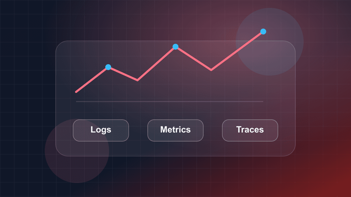
For years, enterprise monitoring vendors popularized the concept of the "Three Pillars of Observability": Metrics, Logs, and Traces. Engineering teams were advised to purchase or deploy three distinct tools:

• A time-series database (e.g., Prometheus, Datadog) for Metrics.
• An inverted-index text store (e.g., Elasticsearch, Logstash, Kibana—the ELK stack, or Splunk) for Logs.
• A distributed tracing collector (e.g., Jaeger, Zipkin) for Traces.

In practice, managing three disconnected telemetry silos creates a fractured diagnostic workflow that actively impedes incident triage.

                    THE DISCONNECTED SILO ANTI-PATTERN
                    
┌──────────────────────┐   ┌──────────────────────┐   ┌──────────────────────┐
│       METRICS        │   │        LOGS          │   │        TRACES        │
│   (Prometheus/TSDB)  │   │     (ELK/Splunk)     │   │   (Jaeger/Zipkin)    │
└──────────┬───────────┘   └──────────┬───────────┘   └──────────┬───────────┘
           │                          │                          │
   Aggregates away all        Text ocean without         Request DAGs without
   request context and        trace correlation;         host metrics or
   high-cardinality tags      slow, expensive regex      resource saturation
           │                          │                          │
           └──────────────────────────┼──────────────────────────┘
                                      ▼
                        Mental Context Switching
                        "Dashboard Graveyard"
                        Manual timestamp matching

Why Disconnected Silos Fail in Production

1. Metrics aggregate away high-cardinality context: Metrics are numeric time-series data points aggregated over time windows (counters, gauges, histograms). While they are computationally efficient for evaluating aggregate rates and triggering threshold alerts, the aggregation process deliberately strips away context. A metric will tell you that the 99th percentile (p99) latency on /api/v1/checkout climbed from $120\text{ms}$ to $4,200\text{ms}$. However, it cannot tell you which specific user_id, shopping_cart_id, tenant_tier, or database_shard caused that elevation.
2. Logs create expensive, unindexed text oceans: Application loggers emit unstructured or semi-structured string messages into stdout or log files. During a cascading failure, a microservice fleet can generate gigabytes of log lines per minute. Without unified request tracing, correlating a single failed transaction across twenty microservices requires manual regex grep queries, timestamp synchronization across servers with drifting clocks, and sheer guesswork. Furthermore, indexing millions of raw text lines in an inverted search index is computationally expensive and memory-intensive.
3. Traces reveal request DAGs but miss underlying machine state: A distributed trace models the lifecycle of a request as a Directed Acyclic Graph (DAG) of spans, recording start times, durations, and network boundaries. While traces show where a request spent its time (e.g., waiting $3,500\text{ms}$ on a database read), an isolated trace cannot tell you if the underlying database host was undergoing a Linux kernel Out-Of-Memory (OOM) memory compaction, saturating its network interface, or experiencing CPU throttling due to container cgroup CPU limits.

The On-Call Incident Workflow in Siloed Environments

When an incident strikes in an organization using disconnected pillars, the on-call engineer experiences the "dashboard graveyard":

1. Alert fires: A Prometheus alert notifications channel reports CheckoutLatencyP99High.
2. Tab 1 (Grafana): The engineer views the latency spike graph. The metric reveals what is happening, but cannot reveal why.
3. Tab 2 (Kibana/Elasticsearch): The engineer opens a log search interface. They enter a time range corresponding to the graph spike and filter by service: checkout-service AND level: ERROR. They encounter 80,000 log lines detailing timeouts, but cannot isolate the initial causal trigger.
4. Tab 3 (Jaeger): The engineer searches for traces with durations $> 3\text{s}$. They find a few spans, but have no way of knowing whether these particular traces represent the statistical cluster driving the p99 metric anomaly or are merely unrelated background tasks.

Every jump between tools requires mental context switching, query translation, and loss of dimensional fidelity.

---

3. The Unified Telemetry Fabric: OpenTelemetry and Exemplars

The modern industry response to silo fragmentation is the Unified Telemetry Fabric, codified by the Cloud Native Computing Foundation's (CNCF) OpenTelemetry (OTel) project.

Instead of treating metrics, logs, and traces as three separate product categories, OpenTelemetry models telemetry as a unified, contextual stream generated from a single instrumented codebase.

                      UNIFIED TELEMETRY FABRIC (OTel)
                      
                         Incoming Request Context
                    (W3C TraceContext: traceparent)
                                   │
                     ┌─────────────┴─────────────┐
                     ▼                           ▼
        ┌─────────────────────────┐ ┌─────────────────────────┐
        │     Active Span         │ │  Histogram Metric Event │
        │ TraceId: 4bf92f3577b34d │ │ Observation: 2,450ms    │
        │ SpanId:  00f067aa0ba902 │ │ (Bucketed into le=2.5s) │
        └────────────┬────────────┘ └────────────┬────────────┘
                     │                           │
                     │    EXEMPLAR ATTACHMENT    │
                     │  (trace_id & span_id      │
                     └──────────────────────────►│
                                                 │
                                                 ▼
                                     Prometheus Metric Sample
                                     + Exemplar: {trace_id, span_id}
                                                 │
                                                 │ 1-Click Jump
                                                 ▼
                                     Trace Waterfall in Tempo
                                     (Span tags, child spans,
                                      correlated log events)

Context Propagation via W3C TraceContext

The foundation of telemetry convergence is standardized context propagation. Under the W3C TraceContext specification, distributed services pass a standardized HTTP header across process boundaries:

traceparent: 00-4bf92f3577b34da6a3ce929d0e0e4736-00f067aa0ba902b7-01

The header encodes:

• Version: 00 (current specification version).
• Trace ID: 4bf92f3577b34da6a3ce929d0e0e4736 (16-byte unique identifier representing the entire end-to-end request transaction).
• Parent ID / Span ID: 00f067aa0ba902b7 (8-byte unique identifier for the immediate upstream caller's span).
• Trace Flags: 01 (bitmask; 01 indicates the trace was sampled for detailed storage).

When every service in an architecture receives and propagates this context, all telemetry emitted during that request's execution—metrics, spans, and structured log records—shares an identical TraceId.

The Critical Bridge: Metric Exemplars

The mechanism connecting aggregated time series to detailed distributed traces is the Exemplar, formalized in the OpenMetrics standard and integrated natively into Prometheus and OpenTelemetry.

An exemplar is a reference to a specific telemetry sample stored outside the metric set, attached directly to a metric measurement. When a metric event occurs (for example, recording an HTTP request duration of $2,450\text{ms}$ into a histogram), the metrics recorder inspects the active execution context. If a distributed trace is active, the metrics library attaches the current trace_id and span_id as an exemplar to that specific histogram bucket:

# TYPE http_request_duration_seconds histogram
http_request_duration_seconds_bucket{le="2.5"} 142 # {trace_id="4bf92f3577b34da6a3ce929d0e0e4736",span_id="00f067aa0ba902b7"} 2.450 1718000000.123

In a modern observability UI (such as Grafana connected to Prometheus and Grafana Tempo):

1. The operator inspects a latency histogram visualization showing an anomalous spike in the p99 bucket.
2. The UI renders clickable dots representing exemplars directly inside the histogram panel.
3. The operator clicks an exemplar point. Without typing a single search query, the UI opens the exact distributed trace waterfall corresponding to that outlier request.
4. The trace shows that the $2,450\text{ms}$ delay was caused by a specific database query lock, complete with the query string and correlated error log events emitted inside that span.

The gap between aggregated monitoring and exploratory observability is bridged with a single click.

---

4. Cardinality and the Time-Series Database (TSDB) Bottleneck

To understand why traditional monitoring tools cannot provide observability, one must examine the internal storage mechanics of Time-Series Databases (TSDBs) like Prometheus, InfluxDB, and M3DB.

Defining Cardinality

In data engineering, cardinality refers to the uniqueness of values contained in a particular dimension or field:

• Low-cardinality attributes: Sets with a small, predictable number of distinct values. Examples: http_method (GET, POST, PUT, DELETE), environment (production, staging), region (us-east-1, eu-west-1), http_status_class (2xx, 4xx, 5xx).
• High-cardinality attributes: Sets with hundreds of thousands, millions, or unbounded distinct values. Examples: user_id, order_id, email, ip_address, session_token, container_instance_id.

The TSDB Cardinality Explosion Formula

In a TSDB such as Prometheus, a distinct time series is instantiated for every unique permutation of a metric name and its label key-value pairs.

If an engineer defines a metric http_requests_total with $k$ label dimensions, the total number of individual time series maintained by the database is given by the Cartesian product of the domain sizes of all labels:

$\text{Total Time Series} = \prod_{i=1}^{k} |D_i|$

Where $|D_i|$ denotes the cardinality (number of distinct values) of label $i$.

Consider a standard low-cardinality metric configuration:

| Dimension Label | Distinct Domain Values | Domain Cardinality $|D_i|$ | | :--- | :--- | :--- | | service_name | checkout, inventory, billing | 3 | | http_method | GET, POST, PUT, DELETE | 4 | | handler | 25 distinct API endpoints | 25 | | status_code | 200, 400, 401, 404, 500 | 5 | | Total Series | $3 \times 4 \times 25 \times 5$ | 1,500 time series |

A workload of 1,500 active time series requires negligible memory and CPU to maintain in a Prometheus TSDB.

Now, suppose a developer attempts to use this monitoring setup for exploratory debugging by adding a single high-cardinality label: user_id, across an active user base of 500,000 users:

$\text{Total Time Series} = 1,500 \times 500,000 = 750,000,000 \text{ time series}$

                THE TSDB CARDINALITY EXPLOSION
                
     Low Cardinality (Safe)              High Cardinality (Crash Loop)
┌──────────────────────────────┐        ┌──────────────────────────────┐
│ http_requests_total{         │        │ http_requests_total{         │
│   service="checkout",        │        │   service="checkout",        │
│   method="POST",             │        │   method="POST",             │
│   status="200"               │   +    │   status="200",              │
│ }                            │        │   user_id="usr_98a7c1" ◄─────┼── 500,000
│                              │        │ }                            │   distinct users
│ 1,500 Active Series          │        │                              │
│ ~15 MB Inverted Index        │        │ 750,000,000 Active Series    │
│ Head chunk memory: minimal   │        │ ~180 GB RAM Index Churn      │
│ CPU: Idle                    │        │ Out-Of-Memory (OOM) Panic    │
└──────────────────────────────┘        └──────────────────────────────┘

Why TSDBs Crash Under High Cardinality

Traditional TSDBs organize data using an inverted index (derived from search engine designs, such as Lucene or Prometheus's block posting lists). For every unique label pair (e.g., user_id="usr_123"), the TSDB allocates:

1. An entry in the dictionary index.
2. A posting list (an array of 32-bit or 64-bit integer series IDs that match that label).
3. An in-memory head chunk buffer (typically storing 120 samples of 16-byte timestamp/float64 pairs).

When series count explodes into the hundreds of millions:

• Memory Exhaustion (OOM): Storing the inverted index postings and open write head chunks consumes hundreds of gigabytes of RAM. The OS kernel invokes the OOM killer, terminating the TSDB process.
• Compaction Thrashing: When the TSDB attempts to flush the two-hour in-memory head block to persistent disk blocks, the disk write amplification and memory required to merge index postings causes disk I/O saturation and database freeze.
• Query Timeouts: Queries requiring label matching must perform set intersections across posting lists containing millions of integers, causing queries to fail with HTTP 504 timeouts.

Because of this architectural constraint, monitoring systems built on traditional TSDBs enforce strict cardinality limits. They forbid attaching request-level attributes. Consequently, they cannot answer questions about specific users, orders, or transactions.

---

5. Wide Columnar Storage: The Engine of Modern Observability

Observability requires arbitrary, ad-hoc querying across high-cardinality attributes. Because traditional inverted-index TSDBs fail at this task, modern observability systems (such as Honeycomb, ClickHouse, and Grafana Loki/Tempo) rely on wide columnar event stores.

TRADITIONAL TSDB (Index-Centric)             COLUMNAR EVENT STORE (Scan-Centric)
Every permutation is a distinct series       Every request is a wide structured row

  Metric Index                               ClickHouse / Honeycomb Table:
┌─────────────────────────────────┐        ┌───────────┬─────────┬───────────┬──────────┐
│ Series ID 1: {method="GET"}     │        │ Timestamp │ Route   │ UserID    │ Latency  │
│ Series ID 2: {method="POST"}    │        ├───────────┼─────────┼───────────┼──────────┤
│ Series ID 3: {user_id="u1"} ◄───┼── OOM  │ 12:00.001 │ /pay    │ usr_981a  │ 142ms    │
│ Series ID 4: {user_id="u2"}     │  Risk  │ 12:00.002 │ /pay    │ usr_332b  │ 2,410ms  │
└─────────────────────────────────┘        │ 12:00.003 │ /cart   │ usr_981a  │ 45ms     │
                                           └───────────┴─────────┴───────────┴──────────┘
                                             ▲ SIMD Vector Scan across millions of rows
                                             ▲ High-ratio column compression (Gorilla/LZ4)
                                             ▲ Zero inverted index overhead for user_id

How Columnar Event Stores Handle High Cardinality

Instead of maintaining an inverted index mapping label permutations to series IDs, a wide columnar event store models telemetry as a flat table of structured events:

1. Physical Storage by Column: Data is stored on disk contiguous by column, not by row. If an event contains 100 attributes (e.g., user_id, ip_address, cart_total, git_commit_sha, cpu_usage), but a diagnostic query only asks for AVG(duration_ms) GROUP BY user_id, the storage engine reads only the duration_ms and user_id byte blocks from disk, bypassing the remaining 98 columns entirely.
2. Columnar Compression Algorithms: Because identical data types are stored sequentially, specialized compression algorithms achieve high data density:
   • Timestamps: Compressed using Delta-of-Delta encoding (as described in the Gorilla paper) or Double-Delta, reducing 64-bit timestamps to less than 1.5 bits per value.
   • High-Cardinality Strings (user_id): Compressed using dictionary encoding (for moderate cardinality) or LZ4/Zstandard block compression, achieving 5x–10x compression ratios.
   • Low-Cardinality Strings (http_method): Replaced with 1-byte integer enumeration tables.
3. Vectorized SIMD Execution: Modern CPUs execute Single Instruction, Multiple Data (SIMD) operations. A columnar database can scan, filter, and aggregate high-cardinality columns at rates exceeding tens of millions of rows per second per CPU core, without requiring pre-computed indexes.

Storage Architecture Comparison

| Architectural Dimension | Traditional TSDB (Prometheus / M3DB) | Inverted-Index Log Store (Elasticsearch) | Wide Columnar Store (ClickHouse / Honeycomb) | | :--- | :--- | :--- | :--- | | Primary Data Model | Numeric time-series vectors ($t, v$) | Text documents with inverted term index | Wide, typed structured event rows | | High-Cardinality Strategy | Strictly forbidden (causes OOM / crash) | Permitted, but causes high RAM usage on doc values | Native design center; arbitrary fields supported | | Write Path Overhead | Low for low cardinality; catastrophic on high cardinality | High CPU and disk I/O due to tokenization and inverted index creation | High write throughput; append-only block sorting and LZ4 compression | | Query Mechanism | Label posting-list intersection | Inverted index search + document retrieval | Linear vector scan over requested columns | | Correlation Model | Separate from logs and traces; requires manual join | Timestamp correlation across text lines | Unified row contains trace ID, span ID, metrics, and tags | | Optimal Use Case | Real-time threshold alerting, low-cost system dashboarding | Full-text arbitrary string search across legacy logs | Exploratory unknown-unknown debugging, multi-tenant analytics |

---

6. SRE Alerting: Moving from Cause-Based Thresholds to Symptom-Based SLOs

The difference between monitoring and observability directly dictates an organization's alerting strategy.

The Failure of Cause-Based Threshold Alerting

Traditional monitoring relies on cause-based threshold alerts. Engineers guess which component failures might occur and configure static limits:

• Alert: HighCPUUsage IF node_cpu_utilization > 85% FOR 10m
• Alert: LowFreeMemory IF node_memory_MemFree_bytes < 1GB FOR 5m
• Alert: DiskWriteQueueHigh IF disk_queue_depth > 10 FOR 15m

In production, cause-based threshold alerting fails in two distinct ways:

1. False Positives (Alert Fatigue): A batch data processing worker or video transcoding service routinely utilizes 98% of available CPU during normal operation. A database server uses 90% of RAM for its InnoDB buffer pool or Postgres shared buffers by design. Paging an engineer at 3:00 AM because CPU exceeded 85% when no end-user experiences degraded service creates alert fatigue, degrading responsiveness during real crises.
2. False Negatives (Undetected Outages): A software update introduces a configuration syntax error in an API gateway routing rule. Incoming checkout requests are immediately rejected with HTTP 404 Not Found status codes. Because the backend service processes zero business logic, its CPU usage drops to 4%, its memory remains stable, and its database queue is empty. Every cause-based alert remains green while 100% of user transactions fail.

Symptom-Based Alerting on SLOs and Error Budgets

Site Reliability Engineering (SRE), pioneered by Google, replaces cause-based threshold alerts with symptom-based alerting tied directly to user experience via Service Level Objectives (SLOs).

1. Service Level Indicator (SLI): A quantifiable metric measuring the level of service provided. It is computed as the ratio of satisfactory events to total valid events:

   $\text{SLI} = \frac{\text{Count of Good Events}}{\text{Count of Total Valid Events}} \times 100\%$

   Example: The percentage of HTTP requests to /api/v1/checkout that return a status code $< 500$ with a server response latency $< 500\text{ms}$.

2. Service Level Objective (SLO): The target reliability agreed upon by business and engineering stakeholders over a rolling compliance window (e.g., 30 days).

   $\text{Target SLO} = 99.9\% \text{ over a 30-day rolling window}$

3. Error Budget: The inverse of the SLO. It represents the total allowable unreliability a service can experience without violating user expectations:

   $\text{Error Budget} = 100\% - \text{SLO} = 100\% - 99.9\% = 0.1\%$

Google SRE Multi-Window Multi-Burn-Rate Alerting

Alerting purely on "error budget remaining" is insufficient: a service could consume 100% of its monthly budget during a 20-minute total outage before an alert fires, or fire prematurely on a 30-second network blip.

The Google SRE framework solves this using Multi-Window Multi-Burn-Rate Alerting.

The burn rate ($b$) is the rate at which a service consumes its error budget relative to its SLO window:

• A burn rate of $b = 1$ means the service will exhaust exactly 100% of its error budget over the course of the 30-day window.
• A burn rate of $b = 14.4$ consumes $2\%$ of the monthly error budget in just 1 hour ($14.4 \times 1\text{h} / (30 \times 24\text{h}) = 2\%$).
• A burn rate of $b = 144$ consumes $10\%$ of the monthly budget in 30 minutes, representing a catastrophic outage.

To eliminate false alarms while guaranteeing rapid reaction times during severe degradations, an alert requires two conditions to be satisfied simultaneously: a short time window (to confirm the degradation is ongoing right now) and a long time window (to verify the burn rate is statistically significant).

                      MULTI-WINDOW BURN-RATE EVALUATION
                      
  Incoming Traffic Stream
            │
            ▼
  Calculate Current SLI:  Good Requests / Total Requests
            │
            ▼
┌───────────────────────────────────────────────────────────────┐
│ Burn Rate Assessment (e.g., Critical Alert Target: b = 14.4)  │
│                                                               │
│   Short Window (2 Minutes):                                   │
│   Is the error budget burning at b >= 14.4 right now?         │
│   [YES] ──► (Prevents waiting if outage is catastrophic)      │
│     │                                                         │
│     ▼                                                         │
│   Long Window (1 Hour):                                       │
│   Has the budget burned at b >= 14.4 over the full hour?      │
│   [YES] ──► (Filters out transient 10-second blips)           │
└───────────────────────────────┬───────────────────────────────┘
                                │
               Both Windows Satisfied Simultaneously?
                                │
               ┌────────────────┴────────────────┐
               ▼                                 ▼
             [YES]                             [NO]
     PAGE ON-CALL ENGINEER              NO INTERRUPT
     (Catastrophic consumption          (Transient anomaly or
      of 2% budget in 1 hour)            acceptable error rate)

| Severity Tier | Budget Consumed | Burn Rate ($b$) | Long Window Duration | Short Window Duration | Paging Action | | :--- | :--- | :--- | :--- | :--- | :--- | | Page (P1) | 2.0% | 14.4 | 1 hour | 5 minutes | Immediate mobile page / on-call wake | | Page (P2) | 5.0% | 6.0 | 6 hours | 30 minutes | Immediate mobile page (day or night) | | Ticket (P3) | 2.0% | 3.0 | 12 hours | 1 hour | Create automated high-priority ticket | | Ticket (P4) | 5.0% | 1.0 | 72 hours | 6 hours | Add to next-business-day triage backlog |

When an SLO multi-burn-rate alert fires, it triggers on user impact (monitoring). The on-call engineer then switches to the system's observability tooling (querying high-cardinality columnar event records and trace waterfalls via exemplars) to determine which component failure caused that burn.

---

7. Implementing Unified Telemetry in TypeScript

The following clean, self-contained, type-safe TypeScript implementation demonstrates the unified telemetry architecture. It establishes:

1. A vendor-neutral telemetry manager modeled after the OpenTelemetry API.
2. Contextual propagation linking distributed trace spans with latency metrics.
3. Exemplar injection binding metric histogram samples to active W3C trace identifiers.
4. High-cardinality structured logging featuring an automated PII (Personally Identifiable Information) redaction pipeline.

/**
 * openstair-telemetry.ts
 * Self-contained, production-grade unified telemetry pipeline.
 * Demonstrates OpenTelemetry-style Spans, Exemplar-linked Metrics,
 * and PII-sanitized High-Cardinality Structured Logging.
 */

import { randomBytes } from "node:crypto";

// --- Domain & Telemetry Types ---

export type TelemetryAttributeValue = string | number | boolean | undefined;
export type TelemetryAttributes = Record<string, TelemetryAttributeValue>;

export interface TraceContext {
  readonly traceId: string; // 16-byte hex (32 characters)
  readonly spanId: string;  // 8-byte hex (16 characters)
  readonly traceFlags: number; // 0x01 = sampled
}

export interface MetricExemplar {
  readonly traceId: string;
  readonly spanId: string;
  readonly timestampMs: number;
  readonly value: number;
}

export interface HistogramBucket {
  readonly upperBoundaryMs: number;
  count: number;
  exemplar?: MetricExemplar;
}

export type LogLevel = "DEBUG" | "INFO" | "WARN" | "ERROR";

export interface StructuredLogRecord {
  readonly timestamp: string;
  readonly level: LogLevel;
  readonly message: string;
  readonly traceContext?: TraceContext;
  readonly attributes: Record<string, unknown>;
}

// --- PII Sanitization Pipeline ---

export class PiiScrubber {
  // Regex patterns for sensitive credentials, emails, and payment card numbers
  private static readonly EMAIL_REGEX = /\b[A-Za-z0-9._%+-]+@[A-Za-z0-9.-]+\.[A-Za-z]{2,}\b/g;
  private static readonly CARD_REGEX = /\b(?:\d{4}[-\s]?){3}\d{4}\b/g;
  private static readonly BEARER_REGEX = /Bearer\s+[A-Za-z0-9\-_.]+/gi;

  public static sanitizeString(input: string): string {
    return input
      .replace(PiiScrubber.BEARER_REGEX, "Bearer [REDACTED_TOKEN]")
      .replace(PiiScrubber.EMAIL_REGEX, "[REDACTED_EMAIL]")
      .replace(PiiScrubber.CARD_REGEX, "[REDACTED_CARD]");
  }

  public static sanitizeAttributes(attrs: Record<string, unknown>): Record<string, unknown> {
    const clean: Record<string, unknown> = {};

    for (const [key, val] of Object.entries(attrs)) {
      const lowerKey = key.toLowerCase();
      // Block known secret keys outright
      if (lowerKey.includes("password") || lowerKey.includes("secret") || lowerKey.includes("token")) {
        clean[key] = "[REDACTED_SENSITIVE]";
        continue;
      }

      if (typeof val === "string") {
        clean[key] = PiiScrubber.sanitizeString(val);
      } else if (val !== null && typeof val === "object" && !Array.isArray(val)) {
        clean[key] = PiiScrubber.sanitizeAttributes(val as Record<string, unknown>);
      } else {
        clean[key] = val;
      }
    }

    return clean;
  }
}

// --- Telemetry Span Implementation ---

export class TelemetrySpan {
  public readonly context: TraceContext;
  public readonly name: string;
  public readonly startTimeMs: number;
  private endTimeMs?: number;
  private readonly attributes: Map<string, TelemetryAttributeValue> = new Map();
  private readonly events: Array<{ name: string; timestampMs: number }> = [];

  constructor(name: string, parentContext?: TraceContext) {
    this.name = name;
    this.startTimeMs = Date.now();

    this.context = {
      traceId: parentContext ? parentContext.traceId : randomBytes(16).toString("hex"),
      spanId: randomBytes(8).toString("hex"),
      traceFlags: 1, // Sampled
    };
  }

  public setAttribute(key: string, value: TelemetryAttributeValue): this {
    this.attributes.set(key, value);
    return this;
  }

  public addEvent(name: string): this {
    this.events.push({ name, timestampMs: Date.now() });
    return this;
  }

  public end(): number {
    this.endTimeMs = Date.now();
    return this.endTimeMs - this.startTimeMs;
  }

  public getDurationMs(): number {
    return (this.endTimeMs ?? Date.now()) - this.startTimeMs;
  }
}

// --- Exemplar-Aware Latency Histogram ---

export class ExemplarHistogram {
  public readonly name: string;
  private readonly buckets: HistogramBucket[];
  private count = 0;
  private sum = 0;

  constructor(name: string, bucketBoundariesMs: number[]) {
    this.name = name;
    // Ensure sorted boundaries and append infinity
    const sorted = [...new Set(bucketBoundariesMs)].sort((a, b) => a - b);
    this.buckets = sorted.map((boundary) => ({ upperBoundaryMs: boundary, count: 0 }));
    this.buckets.push({ upperBoundaryMs: Number.POSITIVE_INFINITY, count: 0 });
  }

  /**
   * Records a latency measurement. If an active trace context is supplied,
   * attaches the traceId and spanId as an OpenMetrics/OpenTelemetry Exemplar.
   */
  public record(valueMs: number, context?: TraceContext): void {
    this.count++;
    this.sum += valueMs;

    for (const bucket of this.buckets) {
      if (valueMs <= bucket.upperBoundaryMs) {
        bucket.count++;

        // Attach an exemplar to the target bucket
        if (context) {
          bucket.exemplar = {
            traceId: context.traceId,
            spanId: context.spanId,
            timestampMs: Date.now(),
            value: valueMs,
          };
        }
        break;
      }
    }
  }

  public getSnapshot(): { count: number; sum: number; buckets: readonly HistogramBucket[] } {
    return {
      count: this.count,
      sum: this.sum,
      buckets: this.buckets.map((b) => ({ ...b })),
    };
  }
}

// --- Unified Telemetry Engine ---

export class UnifiedTelemetryEngine {
  private readonly histogram: ExemplarHistogram;
  private readonly logsSink: StructuredLogRecord[] = [];

  constructor() {
    // Standard latency boundaries: 10ms, 50ms, 100ms, 250ms, 500ms, 1000ms, 2500ms
    this.histogram = new ExemplarHistogram("http_request_duration_ms", [10, 50, 100, 250, 500, 1000, 2500]);
  }

  public startSpan(name: string, parentContext?: TraceContext): TelemetrySpan {
    return new TelemetrySpan(name, parentContext);
  }

  public log(level: LogLevel, message: string, span?: TelemetrySpan, contextAttrs: Record<string, unknown> = {}): void {
    const sanitizedAttrs = PiiScrubber.sanitizeAttributes(contextAttrs);

    const record: StructuredLogRecord = {
      timestamp: new Date().toISOString(),
      level,
      message: PiiScrubber.sanitizeString(message),
      traceContext: span?.context,
      attributes: sanitizedAttrs,
    };

    this.logsSink.push(record);
    // In production, forward to an OLAP columnar collector (ClickHouse, Honeycomb, or Loki)
    console.log(JSON.stringify(record));
  }

  public recordMetric(durationMs: number, span?: TelemetrySpan): void {
    this.histogram.record(durationMs, span?.context);
  }

  public getHistogram(): ExemplarHistogram {
    return this.histogram;
  }

  public getLogs(): readonly StructuredLogRecord[] {
    return this.logsSink;
  }
}

// --- Demonstration: Executing an Observable Transaction ---

export async function processOrderHandler(
  telemetry: UnifiedTelemetryEngine,
  orderPayload: { orderId: string; userEmail: string; amountCents: number; tenantTier: string }
): Promise<{ success: boolean; traceId: string }> {
  // 1. Initialize Root Trace Span
  const rootSpan = telemetry.startSpan("processOrder");
  rootSpan.setAttribute("order.id", orderPayload.orderId);
  rootSpan.setAttribute("tenant.tier", orderPayload.tenantTier);

  telemetry.log("INFO", "Order processing initiated", rootSpan, {
    orderId: orderPayload.orderId,
    customerEmail: orderPayload.userEmail, // Scrubber will mask this automatically
    tenantTier: orderPayload.tenantTier,
  });

  try {
    // 2. Simulate Child Database Operations
    const dbSpan = telemetry.startSpan("db.insertOrder", rootSpan.context);
    dbSpan.setAttribute("db.system", "postgresql");
    
    // Simulate query execution time
    await new Promise((resolve) => setTimeout(resolve, 85));
    dbSpan.end();

    telemetry.log("INFO", "Order persisted to database", dbSpan, {
      orderId: orderPayload.orderId,
      dbDurationMs: dbSpan.getDurationMs(),
    });

    // 3. Complete Root Transaction
    const totalDuration = rootSpan.end();

    // 4. Record Latency Metric with Exemplar linking to the rootSpan context
    telemetry.recordMetric(totalDuration, rootSpan);

    telemetry.log("INFO", "Order processed successfully", rootSpan, {
      totalDurationMs: totalDuration,
      status: "COMPLETED",
    });

    return {
      success: true,
      traceId: rootSpan.context.traceId,
    };
  } catch (error) {
    const totalDuration = rootSpan.end();
    telemetry.recordMetric(totalDuration, rootSpan);

    telemetry.log("ERROR", "Order processing failed", rootSpan, {
      errorMessage: error instanceof Error ? error.message : "Unknown error",
    });

    throw error;
  }
}

---

8. Architectural Comparison: Monitoring vs Observability

To synthesize the differences across system design, operational practices, and tooling choices, the following matrix compares monitoring and observability across eight architectural dimensions:

| Dimension | Monitoring | Observability | | :--- | :--- | :--- | | Fundamental Question | "Is the system healthy according to our pre-configured rules?" | "Why is the system behaving abnormally in this specific cohort?" | | Epistemic Class | Known Unknowns: Tracks conditions anticipated prior to deployment. | Unknown Unknowns: Investigates emergent phenomena never before witnessed. | | System Perspective | External Surveillance: Observes pre-selected outputs against static limits. | State Reconstruction: Infers complete internal state from rich, correlated telemetry. | | Cardinality Support | Low Cardinality Only: Label combinations must remain bounded to prevent TSDB crashes. | High Cardinality Native: Supports arbitrary identifiers (user_id, cart_id, commit_sha). | | Storage Architecture | Inverted-Index TSDB: Time series indexed by posting lists (e.g., Prometheus). | Wide Columnar OLAP: Distributed column-oriented event stores (e.g., ClickHouse). | | Alerting Paradigm | Cause-Based Thresholds: Static alarms (CPU > 85%, Free Disk < 10%). | Symptom-Based SLOs: Multi-window multi-burn-rate alerts on Service Level Objectives. | | Primary Tooling Interface | Static Dashboards: Pre-baked widgets with fixed graphs and dials. | Ad-hoc Query & Flow Engines: Interactive filtering, traces, heatmaps, and exemplar links. | | Debugging Workflow | Jump between siloed tabs (Prometheus $\to$ Kibana $\to$ Jaeger) via manual search. | Direct exemplar drilldown: from an anomalous histogram bucket to the exact trace waterfall. |

---

9. Production Readiness and Architecture Verification Checklist

Before certifying an application's telemetry infrastructure as production-ready, verify your implementation against this architectural checklist:

• [ ] Context Propagation Standardized: Services propagate the W3C traceparent header across all network hops (HTTP, gRPC, Kafka message headers), ensuring distributed causality.
• [ ] Exemplars Enabled in Metrics: Metric histograms and counters capture active trace_id and span_id metadata on samples, enabling one-click drilldowns from latency charts into trace waterfalls.
• [ ] Cardinality Explosion Defenses in Place:
  • TSDB metric labels are strictly validated in CI or linting to prevent dynamic injection of unbounded values (user_id, UUIDs, query strings, timestamps).
  • High-cardinality exploratory attributes are routed to wide columnar event stores (e.g., ClickHouse) or distributed tracing stores rather than metric labels.
• [ ] Symptom-Based Alerting Implemented:
  • Static cause-based threshold alerts (e.g., CPU, memory limits) are downgraded to non-paging diagnostic views.
  • Paging alerts are configured as Multi-Window Multi-Burn-Rate alarms on user-facing Service Level Objectives (SLOs).
• [ ] Automated PII Sanitization Configured: A centralized scrubber sanitizes high-cardinality metadata (masking email addresses, authorization bearer tokens, passwords, and payment card numbers) before telemetry leaves the application process boundary.
• [ ] Sampling Strategy Evaluated: A tail-based or probabilistic head-based sampling strategy is calibrated to retain 100% of error traces and high-latency transactions without incurring prohibitive storage costs during peak traffic.
• [ ] Log-to-Trace Correlation Automated: All structured log records output JSON format and automatically inherit the active TraceId and SpanId from the ambient context.
• [ ] Network Egress and Drop Policies Defined: The telemetry collector (e.g., OpenTelemetry Collector daemonset) has memory limits, buffer backoff strategies, and drop policies defined to prevent telemetry collection from destabilizing the host during network partitions.

---

10. Conclusion

Monitoring and observability are complementary components of a mature reliability engineering strategy, not competitors:

• Monitoring tells you when your system's error budget is burning. It uses efficient, low-cardinality metrics and symptom-based SLO alerts to notify on-call engineers that users are experiencing degradation.
• Observability enables you to diagnose why the budget is burning. It provides the high-cardinality structured events, distributed traces, and exemplar-linked drilldowns required to isolate novel failure modes without deploying emergency code.

Teams that attempt to achieve observability merely by building hundreds of static monitoring dashboards discover that more widgets do not produce faster resolution times. True observability requires designing systems from the ground up to be observable: standardizing context propagation, respecting the storage mechanics of cardinality, eliminating telemetry silos with OpenTelemetry, and grounding alerting in the reality of user experience.

---

Further Reading & Related Architectural Guides

• Backend Observability: Logs, Metrics, Traces, and Alerts — Deep dive into production telemetry collection, OTel collector topologies, and storage engines.
• CI/CD Explained: From Commit to Production — Automated delivery pipelines, canary deployments, and release verification.
• Environment Management Across Development, Staging, and Production — Managing parity, secrets, and configuration boundaries across distributed environments.
• Docker for Developers: Containers Without the Confusion — Container runtime fundamentals, resource isolation, and host metrics.
• Docker Images vs Containers: Understanding the Difference — The architectural distinction between immutable image layers and active execution containers.